This will be a continuation of these notes on precomputed GGX parallax correction, dumping old notes that were never made public before. We are talking stuff I made around 2015!
The TLDR, if you don't want to open the old posts is that we are trying to do the classic precomputed cubemap baked environment lighting. We use mipmaps to encode different preconvolved version of radiance with a GGX kernel of a given roughness. We use Karis/Lazarov's split-sum approximation, make GGX radially symmetric in the precomputation and compensate somewhat.
Lastly, because we're doing state-of-the-art stuff in 2015, we're using proxy geometry to do parallax compensation, so these are not irradiance probes with an infinitely far environment. And we are also renormalizing the probe lighting by the intensity of diffuse probes - a common strategy as typically diffuse probes are dense in space, while specular cubemaps are spatially sparse but high-resolution in the angular domain.
In the previous blog article, what I showed is a bit of reasoning and experimentation around the idea that with parallax correction, the GGX lobe we "bake" in mipmaps becomes "stretched" when we fetch the irradiance, and effectively we have to fit the expected lobe (the one we need in the split-sum BRDF approx) to whatever we baked&stretched in the cubemap.
We could even use a completely different lobe in the cubemap and then somehow do the right fetches and math to reconstruct what we want - because what we want we can't find in the cubemap (after parallax correction) anyways!
Pragmatically, you want a way to "fade out" or "smoothen" the parallax correction at high roughness, because that's where the artifacts become noticeable. For Call of Duty Black Ops 3 we experimented with both, pushing the proxy geometry towards infinity at high roughenss, "smoothing" of the proxy geometry to get rid of the gradient discontinuties (anyways the proxy geo is... a proxy!) and then applying some other math to find the right mipmap to sample.
IMHO, it's really not that interesting to look at the final shader trickery, and I don't remember the exact details anyways. What we want is to understand the problem and the reasoning on how to find solutions.
Now that you are all caught up... let's talk about the occlusion/renormalization!
This time you're in luck...
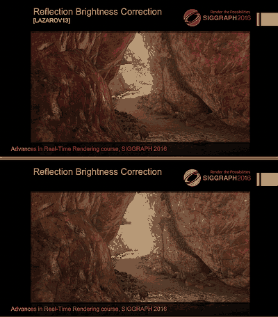
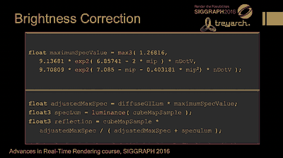
We actually presented all of this. Volumetric GI at Treyarch. There is a comparison slide, and even shader code:
 Old method (on top), new (bottom).
 Shader code. Not 100% sure it's the "right" one.
Do you see it? Do you get it? I don't... This is not to throw shade at the presentation or the presenter (John Hooker), not at all, that slide deck is fantastic and in general, we tried really to be transparent and publish a lot!
It is what it is - presentations are there to inspire you, to encourage discussion in the field, push it forwards... but for a state-of-the-art product, there is no realistic way to reproduce the results simply by following papers/slides, and you constantly have to make tradeoffs between how well you want to explain things, and how many things you can include. And once things go from theory to production, there are a million details that often make a huge difference, but are so specific there is no way to talk about them.
So here we are, before I completely forget the research (I already forgot most of it, but not all) - let's talk about the reasoning behing that screenshot and lines of (dubious) code.
To remind ourselves of the process, the idea of cubemap "renormalization" is to store something like: cubemap_norm = cubemap / diffuse_probe_at_cubemap_position, then in the shader do cubemap = cubemap_norm * diffuse_probe_at_shaded_position. Note I say "something like..." - you might want not to precompute cubemap_norm and instead do everything in the shader, YMMV.
Obviously if we are shading around the point the cubemap was captured, we get the original cubemap back (good), if we are away, the renormalization tries to "guess" what values the cubemap should have had.
The problem we are trying to solve is specular light leaks. This simple renormalization idea just applies a constant multiplier to the entire probe, but irradiance cubemaps can contain quite large amounts of energy emanating from a small set of directions (especially at low-ish roughness), so the multiplier can fail to bring these down enough in shadow areas.
Fresnel makes things even worse - and you end up with the typical artefact of "weirdly bright silouhette edges" - it doesn't help that perceptually light leaks (light where there should not be light) are more noticeable than light over-occlusion.
Effectively what we want to achive is a reconstruction method. We have N signals/inputs that correlate with the values we really want - i.e. irradiance at a specific point in space, from a given set of directions, convolved with a given BRDF - and we want to do some math to approximate these from the inputs - as best as possible.
Often with baked lighting, you have lots of these inputs you want to consider: diffuse probes, diffuse lightmaps, specular probes, various forms of ambient occlusion, various forms of dynamic GI etc... But right now, we limit our inquiry to diffuse/specular probes.
My idea was to think of a "worst case" maximum specular that would be allowed while observing a given local diffuse irradiance. Of course, as a convolution loses, permanently, information, we can't "invert" it, there are many possible radiance/specular configurations of environment lighting that would results in the same diffuse signal, right?
We need an oracle. We need to find a good prior. This is actually a common way of reasoning, when it comes to de-convolving signals.
E.g. in image de-blurring or super-resolution, you know many different images could have produced a given blurred version, but realistically, some inputs are more "natural", more often occurring than others. This is also why deep learning excels at super-resolution, it can effectively learn what things are more probable - the subspace of "natural" images... but I digress - as usual.
Effectively what I was trying to do is the following:
1) We are doing then is to create a model that allows us to go from a diffuse probe to a "fake" radiance probe that would "justify" the diffuse results.
2) From the radiance, we compute (fake) specular irradiance, by convolving with the appropriate GGX lobe
3) Then we can take the maximum value of the fake irradiance probe (we compute everything analytically of course) - and clamp (with a soft-min) the real-but-at-the-wrong-location specular probe values to this value.
As we are clamping, no matter how bright the real specular probe gets, we can always "squash" it down and occlude its values. The only part that we have to finesse what this "fake probe" looks like. We need something that generates a realistic bound, not too conservative to not occlude anything, nor too strict to darken areas that should not be dark. It also needs to be something that in the end we can boil down to a simple formula, it's not that we are going to materialize this fake probe and sample it to get the maximum and so on...
What I did was to assume that all the light we "see" from the diffuse probe (i.e. by querying it at a given direction) is coming from a light direction that would cause the maximum specular response in our case - that's to say, N.V==N.L. We want to obtain a bound for the specular, so this is not a crazy assumption to make.
Then the key was to assume that all that energy does not come from a single direction (that would not generate an useful bound), but instead from a "reasonably" sized area light - a lobe. Because we want analytic/approximated formulas for everything, I "simulated" this area light and its convolution with the GGX lobe as simple mul/add "roughness modification" (i.e. the idea that the GGX specular from a spherical area light looks kind-of like the specular from a single direction, at higher GGX roughness).
Wrap it all up, tie with a bow, and you want to have a formula that, given a roughness, a diffuse scattered value, and n.v, returns the maximum specular value for clamping. Then, because the maths end up still too complex for a shader, you go and further approximate until you get some HLSL that "works" but it is completely devoid of meaning nor usefulness for others :)
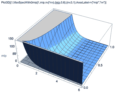
 I can show a million plots like this, they will be fairly meaningless. At least, they are to me.
I could try to reverse the exact experiments I did and the formulas and approximations, but really, I see no value in any of that.
More interesting is to note that the key "tuning" factor in this model is the area light assumption and its "size" - i.e. the tuning of the roughness modification. I ran out of time here and can't claim that there was rigorous fitting of the approximation to data...
What I did was to have a runtime version with parameters I can tune, go around levels and eyeball it.
In theory, one could do this fitting "properly" and at bake time, as each probe corresponds to a given part of the level that might have lighting energy distributed more broadly or narrowly over a small solid angle, and that "area" size should correlate to that. In practice, by now it's all water under the bridge :)
Conclusions
It's all hacks. Physically based rendering, don't tell people, but it's all lies and hacks, even to this day. Sure, we know how to do a few basic things "right", we know reasonable approximations to some other things, but then we start putting things together and approximations are chained in ways that are surely far from optimal, and a lot of the "glue" is complete, undocumented, random hacks.
"Parallax-corrected GGX-prefiltered, diffuse-probe-localized" environment lighting probes (phew that's a mouthfull) are probably among the most hacky of the hacks, but even simpler methods are still very wrong, when you look at them holistically and with any amount of scrutiny... Oh, the BRDF lobe should clamp as it intersects the normal hemisphere horizon you say? Lol...
There is a big opportunity here for whomever is so inclined to claim their name to the next industry-standard method. If someone spent some time actually trying to make a legitimately reasonable, proven, data-driven approximation of the whole thing.
For the rest of you "simply" shipping games, remember that the formulas are not really that meaningful, if you want to be "physically based" you really want to start from the observations. Keep your game in check with real-world measurements first and foremost, and keep groud-truth path-tracers/integrators handy to debug what's going wrong.
If you don't care about real world physics but want to use the "modern" formulas to follow standards and because you heard artists love to be able to reuse assets in different lighting conditions without needing to change material parameters - then you're probably ok without the above mentioned sophistications. But then remember what your objective is... and listen to artists, check their workflows and needs...
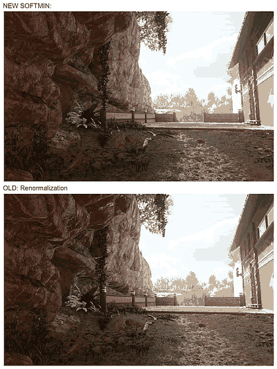
 Some other old A/B tests.

