

Here, we won't be taking the conventional (i.e. good) path to differentiable rendering - there are already a lot of tutorials and libraries about that! E.g. Differentiable rasterization, differentiable path-tracing and most famously, differentiable volumetric rendering (NERFs and Gaussian Splatting).
Instead, we will be building a novel (i.e. bad) way to render differentiably, from scratch, and see what we can learn from it.
- A bit of (personal) history.
I've been interested in machine learning, and specifically automatic code optimization, for more than a decade. In real-time rendering, the name of the game is to find fast approximated solutions to things you can compute by brute force (often trivially), and numerical optimization is a good tool for that.
Near the end of my tenure at Activision, I toyed with the idea of creating an "auto-Jorge" - inspired by the immense amount of work Jorge Jimenez was putting in to refine his state-of-the art techniques, looking at pixels and tuning shaders for quality and performance.
 Pixels this pretty are not easy to craft...
What I wanted to achieve was a way to auto-optimize shader (auto-tune) parameters to aid in the investigation of rendering techniques, at least improving iteration time between idea, coding, and tuning the code enough to understand if a given idea was viable or not.
But long story short, I never got around to really building this out outside some small initial experiments - so I decided to give some of this a try at the end of last year, during our company's "hack week" time!
In particular, I wanted to experiment with modern autodifferentiation systems that have seen an incredible amount of development due to the explosion of deep neural networks, which at their core are all based on gradient descent and thus need the ability to compute derivatives of millions of parameters in complex expressions.
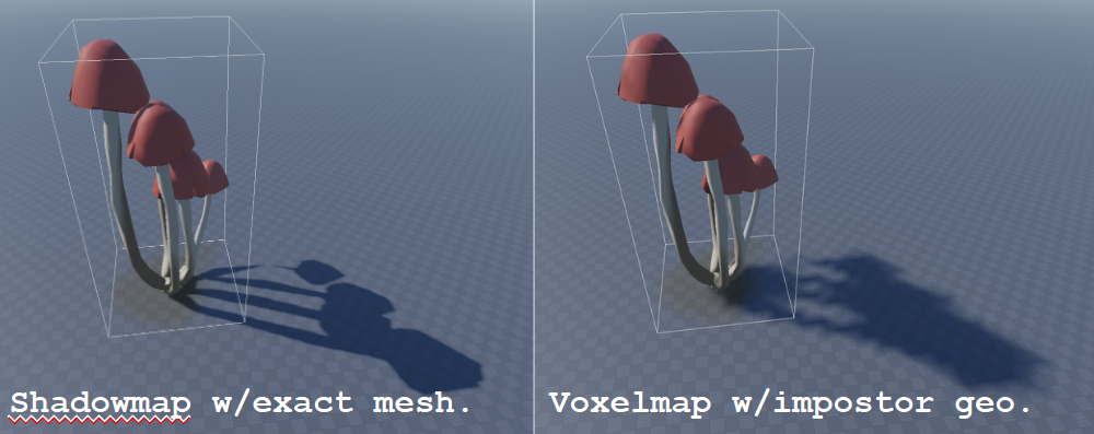
The other reason I was eager to try differentiable rendering specifically is that it connects with some other experiments I've been doing regarding scene simplification. I wrote about some of these in the past already - but we always have new use-cases. For example, recently, we experimented with some ideas of approximating shadow-casting geometry with alternative representation that could be much faster to render; I won't say anything about that today (and should be covered by others anyways; it's not primarily my work), but it's another example where differentiability could potentially help.
The key thing I wanted to make clear in this premise is that I want to test how well autodifferentiation works for complex programs, not build the best possible differential rasterizer - albeit I do think there is some small merit in the approach I've taken.
- Differentiable Rendering 101.
What does it mean to be able to differentiate a program? Well, if you think of a program as a mathematical expression with inputs and outputs, you can then trivially apply any differentiation technique to get partial derivatives of any input with respect to any output - i.e. to know how much a changing a given input would result in a change of a given output.
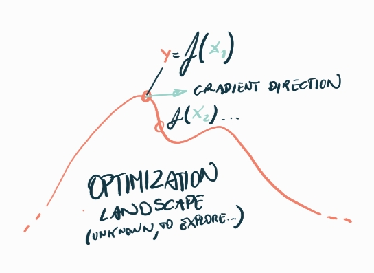
That is the basis of gradient descent - the simplest optimization method that uses derivatives - we take incremental steps of our parameters towards the direction of the gradient in order to minimize or maximize the value of certain outputs.
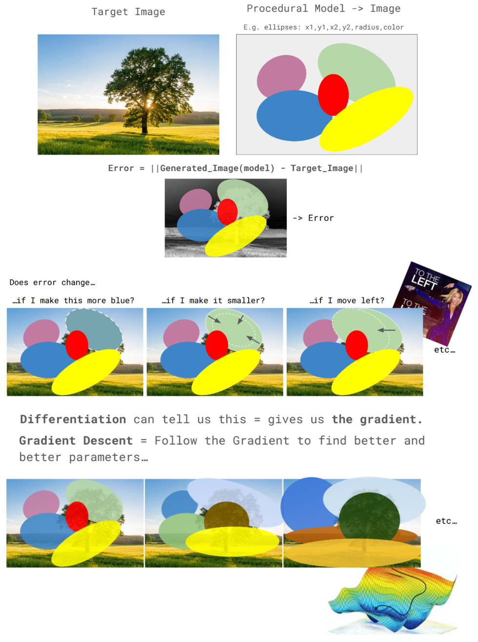
For rendering specifically, we can think of it as a way to generate images from a set of input parameters (a model...). Usually, we can create some reference images (ground truth) that we'd like to match with our renderer. Thus, we can compute an error between the rendered image and the target and use gradient-descent to optimize the model parameters to minimize the error.
 Tl;Dr.
I won't get into how all of this works as tutorials on gradient descent and related methods are a dime a dozen these days, same for how to compute derivatives automatically via the chain rule (a.k.a. "backpropagation") or dual numbers ("forward-mode differentiation"). Just as a reminder, all this mechanism is handy when we have a ton of dimensions (parameters) to optimize, as in these scenarios, we can't imagine just "looking around" (gradient-free optimization) the parameter space to decide where to go, the number of potential roads we can take is too high (curse of dimensionality).
If any of this sounds unfamiliar, search "gradient descent" (versus gradient-free optimiation methods), "automatic differentiation", "backpropagation" (versus dual-numbers, symbolic differentiation and finite differencing) to get up to speed. Or ask your favorite LLM to "Make a small Python program that uses Jax to fit a sum of a number of 2d Gaussians, specified by their x,y center, amplitude and 2d covariance matrix, to a grayscale target image" and learn by doing (a copy and paste)! :)
- Dealing with discontinuities.
But, of course, a program is not an algebraic expression, right? It contains control flow! And even the parts that do not can still very well not be differentiable (i.e. have discontinuities). So, how would we compute gradients for these?
Well, first of all, let me tell you that this might not be a problem at all!
Let's think of one of the simplest discontinuities in a program, a conditional move, like C/C++ ternary operator: x=cond?a:b. We can still compute the derivatives when we land on one side or the other of the conditional - remember that our derivatives are numerical and evaluated at a given point, we are not writing down the symbolic representation of them (which, in general, would be more expensive to compute).
The fact that the derivatives don't "see" the conditional (has zero gradient) just makes the optimization "blind" to it: we wouldn't know that taking a step that would change the result of the conditional has the potential to change the output in a given way - but this does not break the system per-se!
This holds true in general, even for control flow like branches and loops, your function could change at each step during the optimization, and automatic differentiation would still work, but gradient descent might not then be the best strategy.
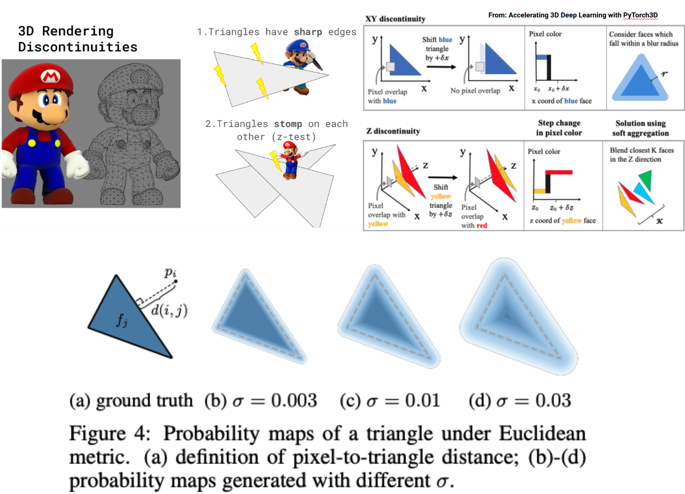
Ok, but what if you want to make gradient "see through" these discontinuities - i.e. they are important to optimize our parameters? Well, the simplest solution is just to replace them with smooth functions to provide a bit of a gradient (if you want, you can think of making the logic of your program "fuzzy" - associated with a smooth probability of taking a branch, instead of a step function). Of course, this changes the results of the program, and thus, there is a tradeoff between how much you "smoothen" the discontinuities and the ability to minimize the error function with respect to the original program, but if you smoothen just the "right amount" - it works!
In Computer Graphics, especially if you are a bit old-school, we're used to these manipulations! Replacing control flow with conditional moves was (and to some degrees still is) a good trick, as dynamic branches can be expensive for GPUs (or impossible if differentials are needed). And then "smoothing" these conditional moves (step functions) can be a good idea to lessen shader aliasing issues (you can learn the math to analytically antialias - convolve with a given pixel kernel - albeit, nobody does these things anymore).
And this idea of smoothing a program is how conventional differentiable rasterization works: edge equations are trivial to smooth, depth-test is a bit trickier but similar.
In general, we modify the rasterizer to save a number of fragments per pixel - this is needed as now the edges are "blurry" - then write a function to "resolve" them. That could be done by averaging the depths or other similar ideas or even just sorting and taking the frontmost. That would mean that the gradient would not be sensitive to the fact that moving a primitive might result in a different depth-test outcome (a different primitive becoming visible for certain pixels), but that is not a big deal, we would "see" the new results in the next optimization step, and if we optimize from different points of view, the front-back movement in one view can be seen as an x-y in another, and the latter is differentiable!
 Smooth your edges!
- A new challenger is approaching!
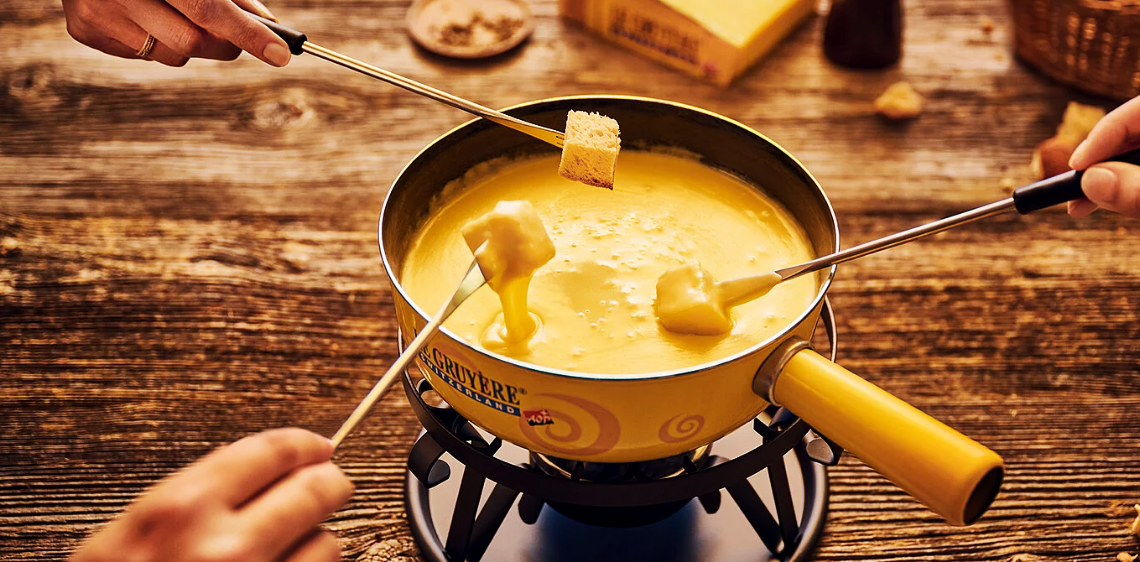 A fonduational model.
Ok, but so far, we have been re-threading (badly) known stuff. Where's the novelty? Here it comes. After observing that the best differentiable rendering starts from formulating the problem in a way that is "naturally soft," like NERFs and Gaussian Splatting do with volumetric rendering, I wondered - what it would look like to make a depth-buffer that is naturally always soft?
As a thought experiment... if you take a depth-buffer and blur it, what do you get? A height-field of sorts, where all sharp object boundaries become slopes. I call this idea "blanket-rendering" or "fondue-rendering":
Now, I won't keep teasing it because the idea is trivial, and most of you already spotted it, as I imagine every one of the people potentially reading this is versed in ShaderToy... Sphere-tracing (a.k.a. SDF raymarching)!
One of its main issues... I mean, useful properties... is that it "slows down" marching near primitive edges, and thus it naturally results in a continuous, smooth rendering.
Normally, we want to minimize this effect by doing enough iterations in our marching loop and by putting other "smarts" in the loop, like early-exits or heuristics to "over-step" and backtrack, but here, we'd be exploiting this property to gain differentiability.
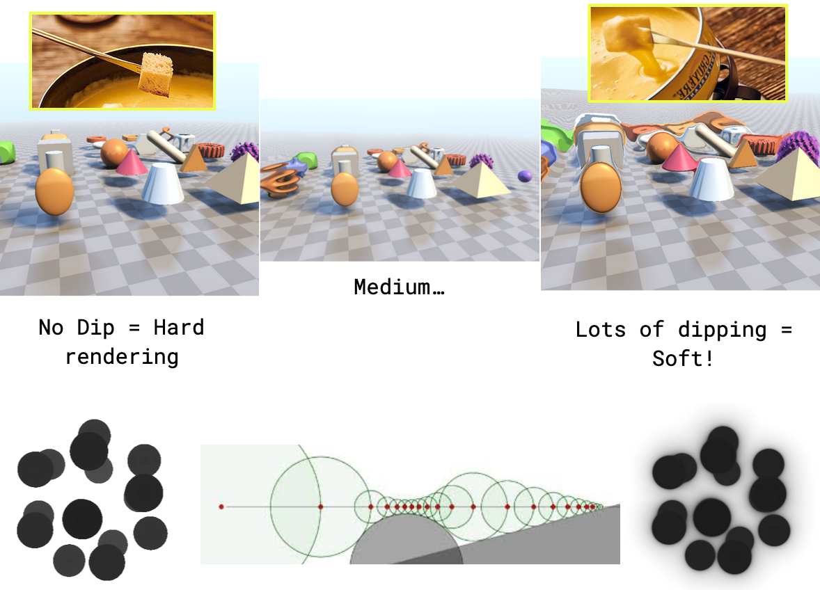
It's really as simple as this. I made a basic sphere-tracing raymarcher in shadertoy, I then made sure it was "soft" by removing most branches and avoiding to march "too much" in the main loop (note that the marching loop, as it is over a constant number of iterations, does not cause discontinuities at all, you can just unroll it and have no control flow), and factored the parameters of the primitives I wanted to optimize in an array that I passed to the marching function.
Then I just took the whole thing, copy-pasted in an LLM, and asked it to translate from GLSL to Python using Jax - et voila! A rasterizer written in Python/Jax ready to be differentiated!
All of the plumbing from here on can also be done by LLM code assist: telling Jax that we indeed want to differentiate the scene parameters (sphere positions and radii), plugging in an error function, and doing gradient descent.
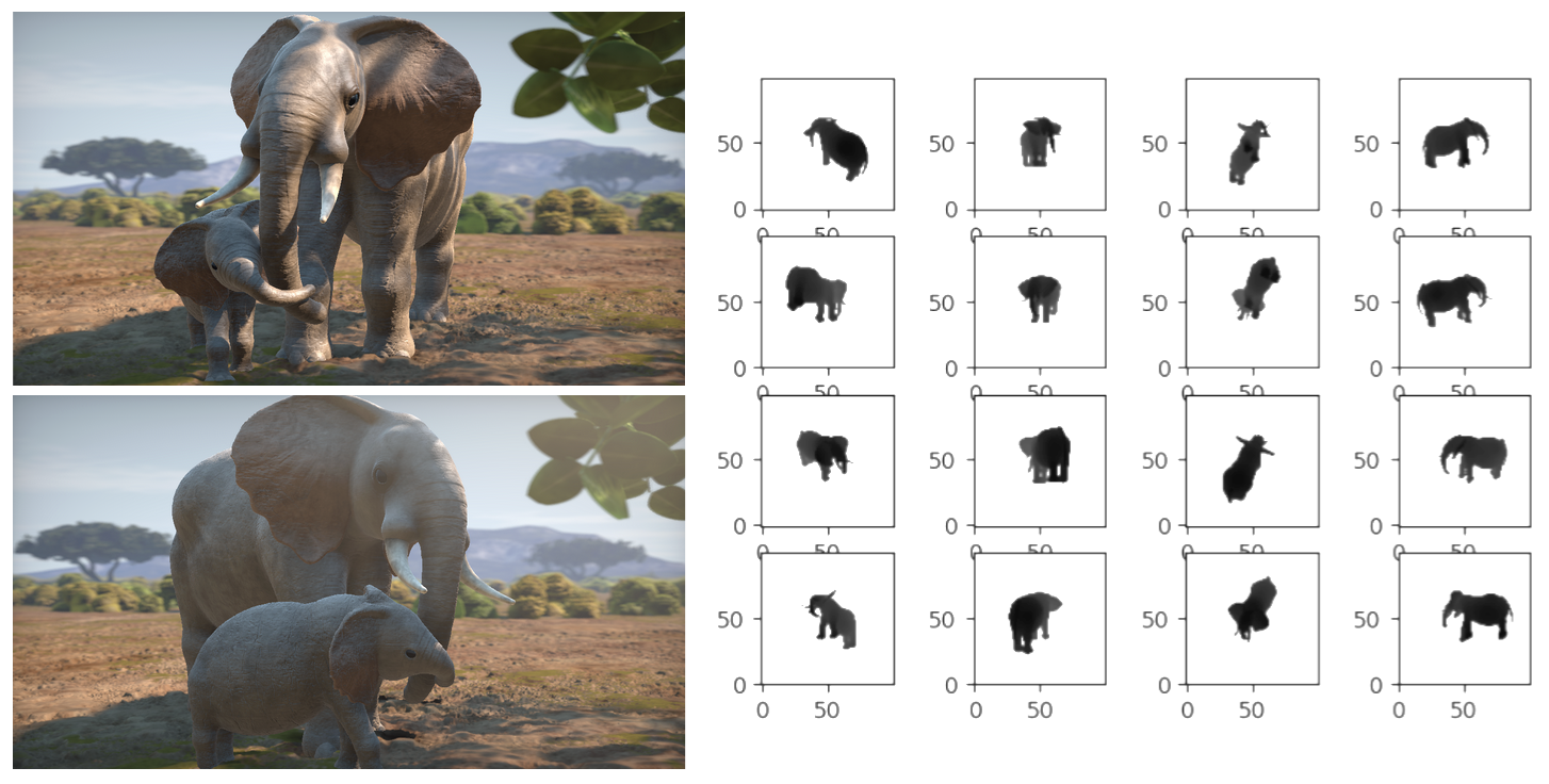
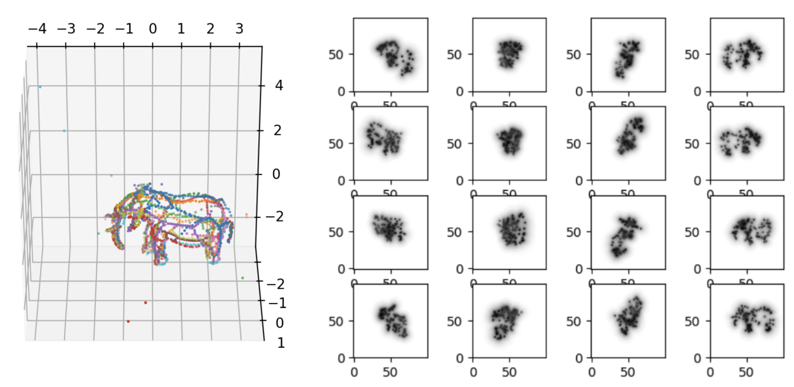
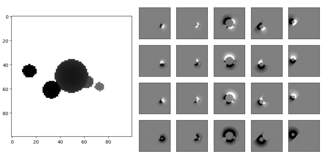 A depth buffer produced by rendering five spheres via SDF marching, and the per-pixel gradients of each parameter.
You can see in the image above the output of the "forward pass" of the raymarcher: a depth buffer, and a matrix of images where each column corresponds to one of the five spheres in the scene, and each row to one of each of the sphere's parameters (x,y,z,radius), visualizing the per-pixel gradient - i.e. how the scene depth would change given a change of that specific parameter.
Once we plug in an error function, comparing a reference scene depth to our model's output depth, we'll get a gradient where each entry of that matrix is a single float - i.e. how the error would change given a change of one of the parameters, and that can be used directly to iterate towards the direction of minimum error. Gradient descent!
There are a few caveats here and there, but for the most part, it's just that simple. The idea here is that we'd like to approximate a complex scene with a few primitives. We only need to generate depth buffers from a number of viewpoints, of the target scene, and that can be done with any rendering technique, it does not need to be the same as we use for the differentiable rendering.
The output depths have to have, obviously, the same meaning - to be in the same coordinate system.
For convenience here, I used shadertoy again, searched for "IQ" and shamelessly ripped the first scene that looked like it could be a good target for this.
Again, after working in shadertoy a bit to simplify the code and remove all the bits and pieces I did not need, I just asked an LLM to do the conversion from GLSL to Python to have everything in the same system. Again, I used Jax here, albeit, as we don't need derivatives here, I could have used anything else, from pure Python to NumPy, etc.
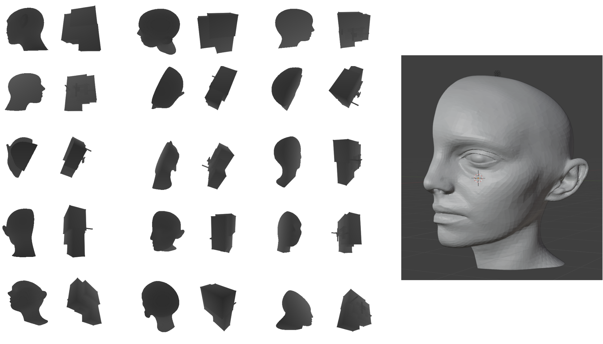
 My test scene, rendered from several fixed views.
Now, for the optimization to work, you could keep generating viewpoints on the fly, randomly or with low-discrepancy sequences (on a sphere or hemisphere around the virtual object) - at each iteration selecting a new viewpoint, and we can call this "stochastic gradient descent" as now we work with random subsets of data ("batches").
In practice, I just pre-rendered the target scene from a small number of fixed viewpoints (16 seemed enough; I used a spherical T-design to be fancy) and iterated through these in the optimization loop.
Note - One of the caveats is that due to the nature of the fixed-step marching, the "far plane" in our renderer is implicit, the depth won't ever be bigger than NEAR_PLANE + NUM_STEP * MAX_STEP_SIZE. I suggest explicitly clamping the distance function with such a MAX_STEP_SIZE; it helps with making sphere-tracing "softer." As an alternative, one could avoid that, take fewer steps, and use a max or soft-max to impose a far-plane.
It's then important to match the reference depth buffers far-plane to whatever our raymarcher will generate, otherwise, there will always be areas of large error in the background (albeit they should not influence the gradient).
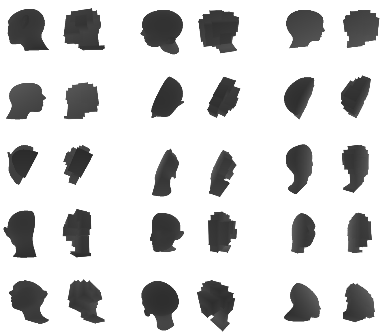
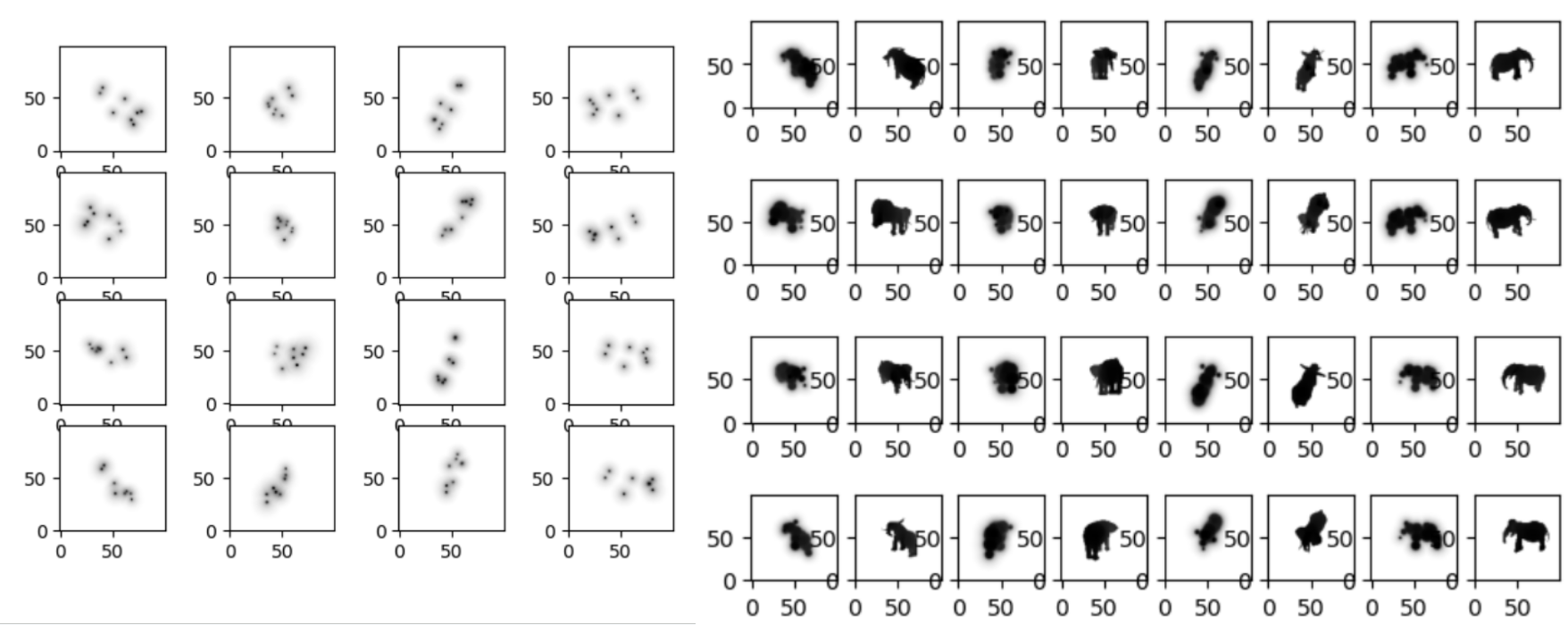 Some randomly initialized spheres (left), and then converged and compared to the target views (right).
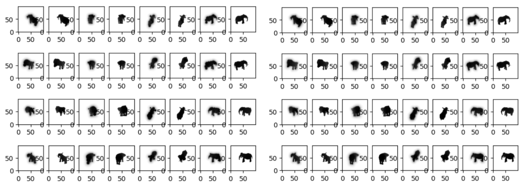 Converged results with 32 primitives (left) and 100 (right).
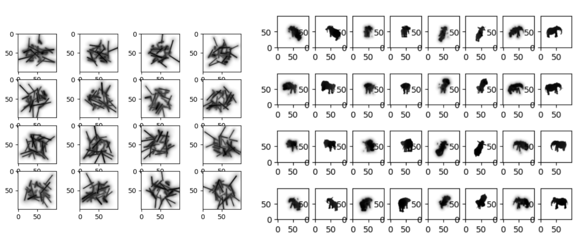 We can also use other primitives, of course. Here, trying with 32 single-radius "capsules".
And this... kind of just... works. You can see some of the results above.
- Digression: Jax versus PyTorch and alternatives.
Before we go into some more (important) details and optimizations, a digression: so far, I've mentioned I've been doing all of this with "Jax" and that LLMs translated everything by magic for me. And it is mostly true, but not entirely - in general, it's good to know a bit more of what's going on.
Google's Jax, like Meta's PyTorch, is a library that centers around a vector data type. Effectively, they both provide a drop-in replacement for NumPy - you write Python code in NumPy style (which is to say, in an array-programming style, NumPy is inspired by APL, Fortran, Matlab etc...), and by "magic," you get differentiation and other useful transformations.
This "magic" is, in both cases, similar. Both libraries trace python code, interpret it, and "follow" the interpretation to record what was going on in their own intermediate language - that's what enables them from there on to do autodifferentiation.
This interpretation step is used to annotate the types of all variables (specifically the dimensions and types of the vectors, as Python/NumPy code is not statically typed) and to navigate all control flow that is not predicated on the vectors that we want to differentiate.
Where the two libraries differ significantly is in how the forward and backward (gradient) execution proceeds. From what I understand, PyTorch always interprets its intermediate language, even if it has some functionality to "precompile" and "JIT" these terms always refer to the creation of the IL from Python, not to how the IL is executed or how the gradient step would proceed (which requires to emit a trace from the IL to walk backward).
PyTorch idea is to use Python code instead of having programmers explicitly build a computation graph using differentiable "blocks", like it is/was with TensorFlow, but it is still made with the idea that you'd use few, big functions, like neural-network layers, that have the forward and backward evaluation optimized in native code.
In contrast, Jax is always compiled to native code, even if it superficially looks similar. In fact, you can provide manually the type information and trigger a compilation, but it can even just do everything "by magic" behind the scenes, triggering a compilation any time it thinks it's needed.
One can even provide a list of variables that are meant to be constant during a given execution, and Jax will hash their values and compile specialized code per each variant it encounters. You can even ask Jax to dump all the generated code and the various intermediate steps it takes - all eventually ending in LLVM IR - kind of like you do when debugging shader compilation...
This is tremendously faster for differentiable programming of long, complex code (like in our case...), but even if it mostly works by magic, there are a few things to be aware of. First, Jax can't branch (python if statements...) with predicates that involve Jax "traced" arrays. Use the "where" function instead (similar to a conditional move). This is because, from the perspective of the traced code, the computation has always to be static!
Second, Jax will always trace through Python control flow, loops, branches, etc, but this does not mean it's the ideal way! In particular, for loops, this results in unrolling the loop in Jax's internal representation, which can slow down the compilation. The only real problem I had with Jax is that at a given point, when trying to compile Inigo's shader translated to it, it would just time out.
To ameliorate this, you can instead use Jax's own functional programming operations to express the flow: map, vmap, for_i_loop. Vmap is, like the name hints, a vectorized map that tries to evaluate a given function in parallel, use that wisely! It can speed up inner loops, but it can be too much if used outside large code.
Lastly, although Jax's vectors have most of NumPy's function, beware that most linear algebra functions are optimized for large vectors and matrices, unlike what we usually deal with in 3d graphics. For example, the LLM I was using converted GLSL normalize() to Jax jnp.linalg.norm, which worked correctly but bloated the generated code horribly.
Autodidax and Jax the sharp bits are great reads!
- Global Optimization!
Let's go back to our differential rasterizer and using it to approximate a known scene with a given number of primitives... I said, and have shown that it works. And that's true... if you don't look closely. I mean, that's how you write papers, right? But this is not a paper, so let's reveal the ugly truth!
If we render, using good old "hard" rendering, the original object and its approximation, we can notice that it's not that great:
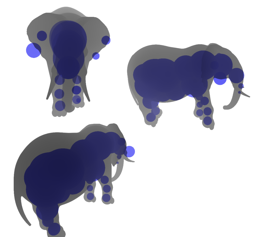 Comparison of the original elephant and its approximation. Using 32 primitives.
What's going on here? There are two issues, one minor, the other one not-so-minor. The former is that the "softening" that we need to use to get gradients makes the differentiably-rendered primitives "thinner" than the equivalent primitives in "hard" rendering (e.g. raytracing).
This is not a big deal, in fact, it was again mostly due to laziness/time that I did not fix it: with a system like this, the ideal would be to "harden" the renderer as the optimization progresses. Softer rendering at the beginning means that even if a primitive is far from the regions of the scene it should move towards, it can "catch" them, it will have a larger radius of pixels around it that is influenced by it - and thus, captured in its gradient, but once the primitives "settle" in their regions, there is no need of that anymore.
The second and bigger issue is that gradient descent is, at best, a local optimizer (i.e. it will find a local minima), but our problem has multiple minima, and many of them are terrible. For example, imagine initializing all the primitives in such a way they are not visible at all, they are either too small or past the near/far planes, and so on. That is a minimum, the gradient will be zero, no change can be seen that improves the error, and yet, clearly, it's a terrible minimum. Same if multiple primitives are "buried" inside others, these will never be visible from any point of view, their gradients will be zero, and yet they will be far from where they should optimally be...
In general, if the primitives are initialized "badly", e.g. they start far from the areas they should be, then they will converge somewhere near the model but not with the right density, too many primitives can be used to approximate minor details, whilst none will be available to converge in other areas that have high error.
This is the opposite of what happens with large, deep neural networks, where we want to optimize with lots of parameters, even just in the hope that some will be randomly initialized in "good" ways, and getting near any local minima is good enough. Then, we can even "prune" away the parameters we didn't really need.
This problem requires ideally starting from an already decent solution, derived through other means, and use gradients only to optimize further (no surprise, by the way, this is how Gaussian Splatting works too!). Or, if that's not possible, we need to use either global optimization or at least some systems to control the primitive placement over time, removing primitives if they start to be too dense in areas of low error and adding them in areas where we still have high error (and again, no surprise, Gaussian Splatting does that too)! We can also think of ways to inject some penalty terms in the error function to penalize primitive distributions that are not ideal - for example, avoid compenetration or too small primitives.
These are all things that require time to experiment with, I've played only with a few basic techniques (a few extra lines of code, really) and will show how big of a difference they make.
First, I have to say that even in the "naive" experiments I've shown so far, a modicum of care was taken. I initialize the primitives to be randomly distributed "around" the object (e.g. in a sphere), and I make them "small" at first so that there is no compenetration/burying of primitives. I also, at each iteration, check for primitives that vanished (became too small) and randomly re-initialize them.
 Better initialization.
I then thought I could quickly write something that would compute an approximation of the target shape medial axis, sample points over it, and then from these take a few as the primitive centers, using Mitchell's best-cadidate algorithm to pick well-spaced ones.
This worked decently, but it also had errors I didn't care to fix further, as I knew that if you have a way to generate a good initial solution, then for sure you can get a good approximation. I thus moved to exploring ideas of how to improve the optimization algorithm instead.
Here is also where I switched from my raymarched differential renderer to a more conventional, triangle-based, differentiable rasterizer - namely, PyTorch3d (which, btw, was somewhat of a pain to install, ML python packages tend to require arcane incantations to resolve their dependencies as they evolve fast and rely on a ton of other modules - and luckily I already had a working WSL2-miniconda environment with Cuda and PyTorch et al! On the bright side, once setup, WSL2 worked like a charm, and I could develop using VSCode's "remote" connection to the local VM, never having to touch Linux further).
This mostly to play with more useful tech, to remove from the equation other errors and things to tune in my own system, and because I never bothered to enable GPU acceleration in Jax, and thus the system was relatively (but not terribly) slow, having to render everything on CPU.
 Recreating a similar setup as with my own renderer, using PyTorch3d.
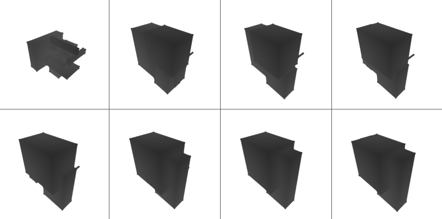 Solution evolving over time (visualized from a single, fixed viewpoint).
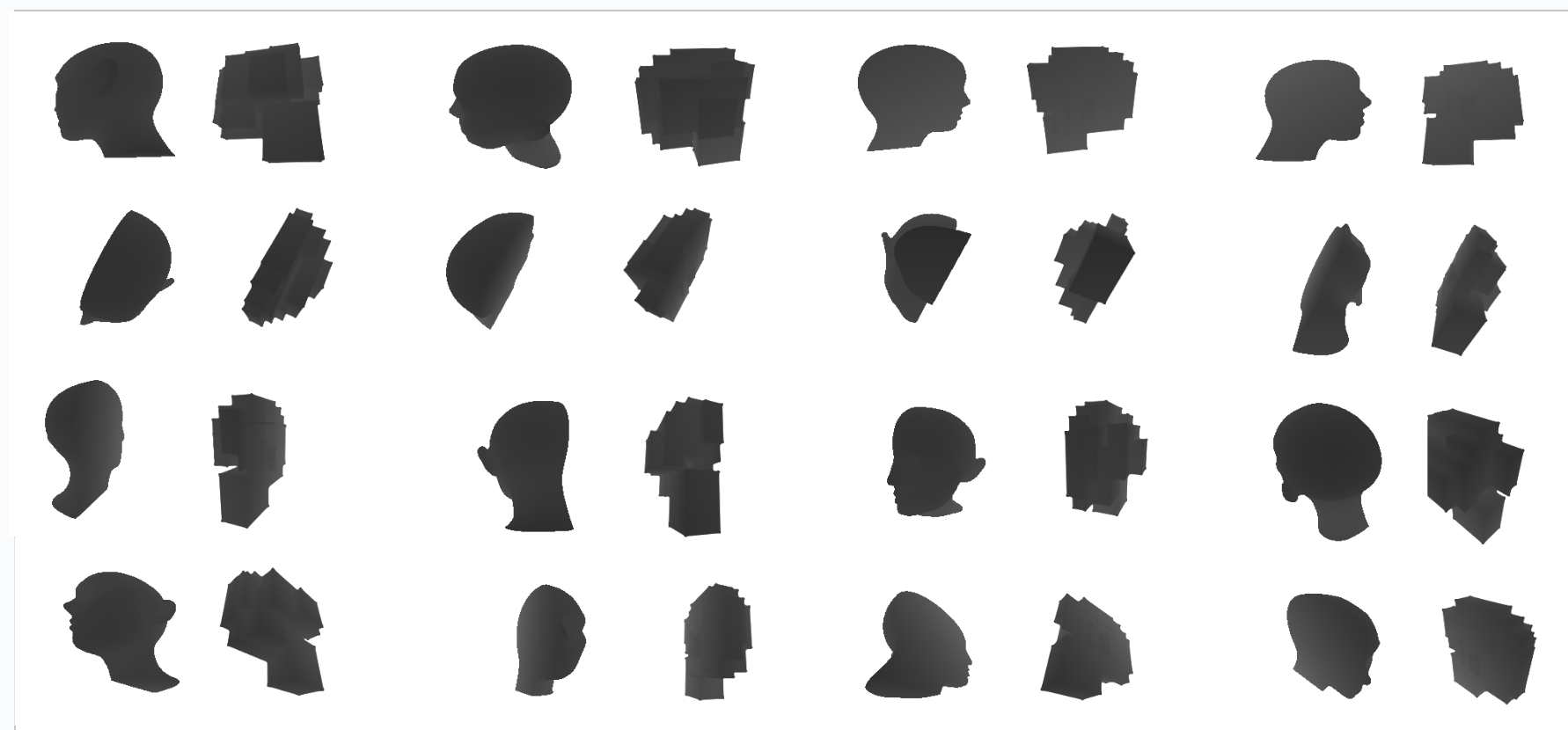
Instead of spheres or capsules here I used AABBs - for a change, and I generated the reference depth buffers by simply rendering an object I loaded from a Wavefront .obj I had "lying around". You can see that in the image above, where I employ only gradient descent and randomly initialized boxes, we converge towards a decent result, but many primitives end up being "wasted": too thin/small, too dense in certain regions while sparse in others...
Note that PyTorch3d, even if it is a triangle-based differentiable rasterizer, does not imply you have to optimize individual mesh vertices. You can generate a mesh from a set of parameters, and because a program is a program and differentiation works over generic code, the parameters that generate the mesh can be subject to gradient descent! And because the program is a relatively small Python script that "plugs" into a differentiable black box, PyTorch interpretation overhead does not matter.
The first test I made was to add a global optimizer to the mix, specifically, Genetic Programming. Population-based methods and evolutionary algorithms, in particular, seemed perfect for this use case. Specifically, for cross-over (mixing two solutions to produce a new one by taking parts of one and parts of the other) to work well, the problem should fulfill the "Building Block Hypothesis (BBH)" - the problem's solution space should have useful, reusable building blocks that can be combined to create increasingly optimal solutions. This is obviously true in our case, if certain primitives are converged to good areas, these represent "reusable building blocks", and GP should work well.
The idea here is simple. I keep a small population of candidate solutions. I then quickly optimize them using a few iterations of gradient descent (it doesn't matter to converge at all - anyways, we'll iterate more over the next population) and record their final error.
Then, I use the standard GP idea to produce a new set of candidate solutions by taking the best found in the previous generation, remixing them (swapping certain primitive parameters using crossover), rinse and repeat. This works... fantastically well, even without having done extensive tuning of the GP method, and it is much faster than trying to use GP alone!
 Still 16 AABBs, but much, much better!
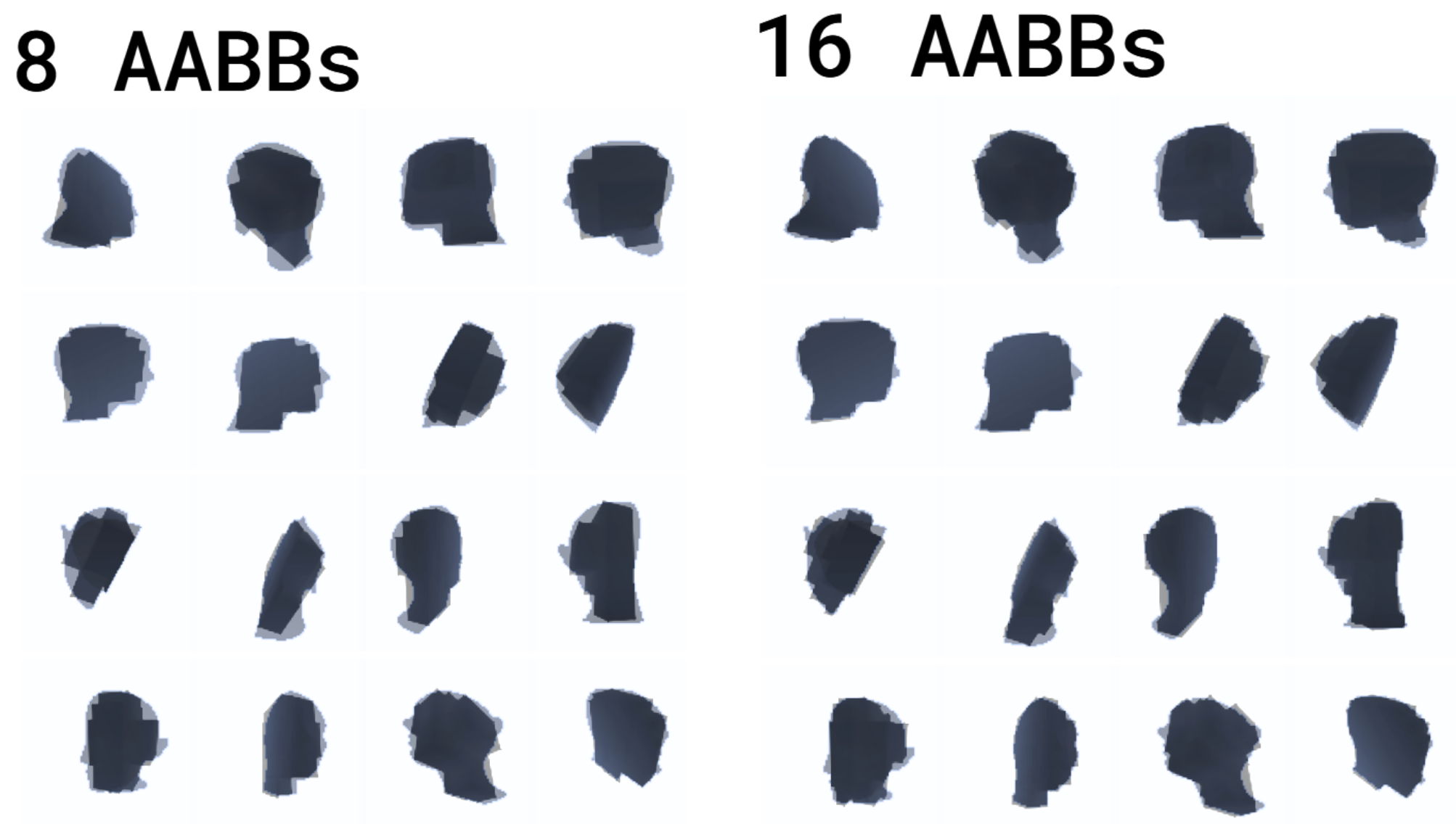 Different runs, rendered overlaid with the original mesh.
- Hierarchial splits.
Next, and last, I tried another idea I knew would improve the results drastically: hierarchical splitting. Simply put, instead of trying to directly optimize the target number of primitives, which makes it very sensitive to how we initialize them, we start from the simplest possible case: just one primitive.
If you think about it - with one primitive, you have only one global optima (minus possible symmetries in the solution, i.e. if swapping the min and max of the AABB corner parameters still produces the same AABB), so gradient descent should be able to find it if we initialize the solution even half-decently (e.g. computing the AABB of the target object, or even just its centroid - or even just being in the general vicinity of the object!).
Then, after we converge, we can add one more primitive by finding the one in the solution that has the biggest error from the area it's approximating and splitting it. Ideally, splitting it over the axis that "helps" the error the most, which we could do if, for example, we compute said error over the primitive faces, or edges/vertices etc.
In my case, again, lazy/no time, I just took the biggest primitive and divided it along its longest axis... Far from ideal, but still:
 16 AABBs, optimized with hierarchical splitting.
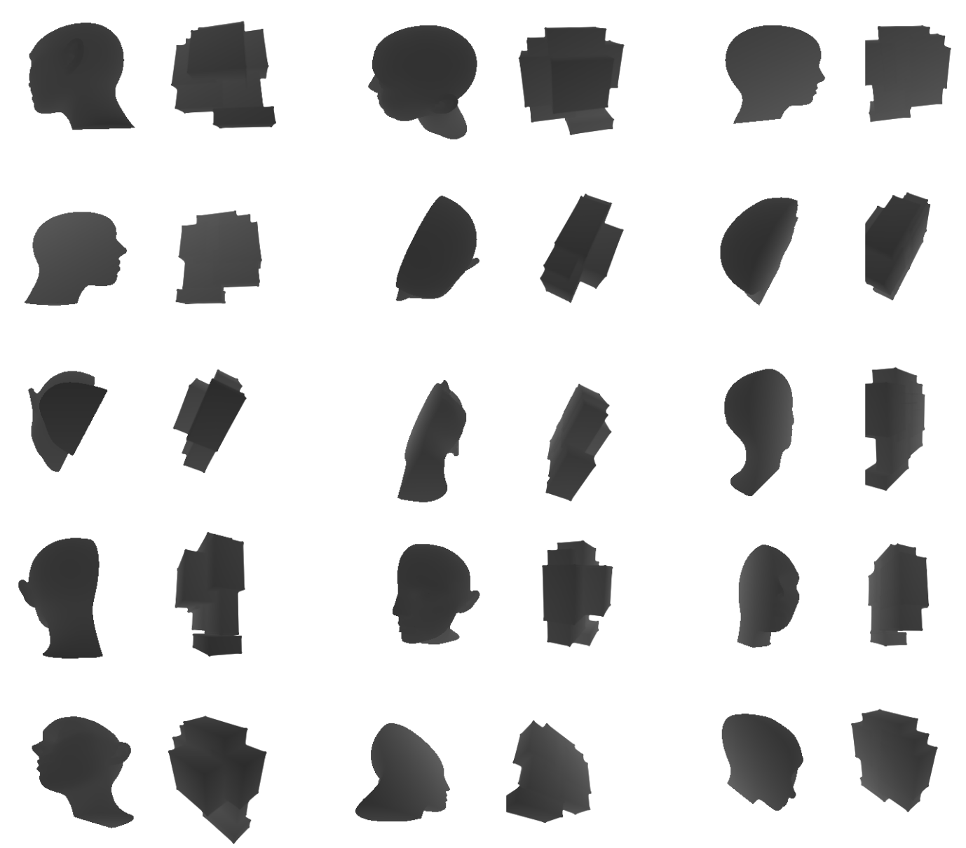 Same, but with only 8 AABBs.
Very good results, and very fast!
- Conclusions.
So, what did we do, and what did we learn from this?
1) We made our very own differentiable renderer, from scratch.
Yes, it might not be the best (for example, it would be tough to support shading; it really works only for shape optimization, e.g. depth only), but it works, it's fast, and arguably might have some advantages over rasterization. For example, it doesn't need much memory as it never needs to store multiple fragments to then blend them. It's also ray-based, so we could sample the image sparsely, we could cast secondary rays, and so on.
2) We learned that modern auto-differentiation systems can cope with complex, almost arbitrary programs.
Jax worked very well after learning about a few caveats, and I suspect that Mitsuba's Dr.Jit, which was made specifically for graphics code (i.e. lots of code dealing with small vectors) might be even better.
One day, I still dream of being able to autodifferentiate/autotune shaders directly - to hit given quality and performance metrics (multi-objective optimization), and being able to specify what's continuous enough to use gradient descent, what parameters should be considered as discrete code alternative to optimize combinatorally, what parameters might need continuous but noisy optimization, which ones need constrained optimization and so on. I think this is very doable, just requires some time, and in my dreams I imagine that certain parts of a shader could even be tagged as "auto-generate code here", for black-box methods, symbolic regression and the like.
3) Initialization, heuristics to guide gradient descent, and global optimization matter...
...for non-deep model. Duh! Next, I'll tell you that "feature engineering" matters as well - this is all known, but at least we saw it in practice!
4) Lots of problems could be solved better (simpler/to highest-quality solutions) with a bit of gradient descent.
If you have a good starting solution provided by a conventional algorithm, it should be easy to sprinkle some GD-based post-processing to improve it!
If I had more time... next time...
- I'd want to build the system I mentioned in (2) above.
- I'd be interested in trying to see if, instead of depth-averaging, recording depth statistics (moments et similia) could be used.
- It would be neat to joint-optimize LOD everything: geometry and textures, but this has already been done :) (see also)
- I think it would be especially interesting to generate approximate occlusion meshes, as that is a hard thing to do geometrically. In particular, there is this 2014 paper by Ari S., which always intrigued me but also seemed complex in practice, and I think it could be much easier with differentiable rendering. It should not be hard to write a differentiable renderer that "slices" a mesh (e.g. by sampling a SDF generated from it) or even just directly force our approximation primitives to be subdivided planes/disks with a few vertices and optimize the vertex position on the plane jointly with the plane parameters. The interesting thing is that with numerical methods, penalizing more if the approximated shape lies outside the model (to have conservative occluders) is trivial!